Table of Contents
- Introduction
- Mechanics of Dot Products
- Transformer Architecture (Encoder-Decoder)
- Self-Attention in Detail
- Role of the Feed-Forward Network in a Transformer
- The Decoder, Final Layer & Softmax
- GPT-2 Architecture — Decoder Only
- Complications with Eigen — The Rowwise & Colwise Mess
- A Few Pretty Graphs & Conclusions
1. Introduction
For the past five years, Claude, ChatGPT, and Gemini have been everywhere. Engineering, finance, marketing — pick a field, there’s a model in it. Most people using these tools don’t think too hard about what’s actually happening under the hood. And honestly, fair enough. But all of it — every summarization, every code completion, every agentic workflow where a model picks up tools and starts acting — goes back to a single 2017 paper: Attention is All You Need.
For someone with ADHD, that title hit different. Attention is quite literally what I have been fighting for my entire life. Pun very much intended.
The idea that a mechanism called “attention” could turn next-token prediction into a general-purpose reasoning engine is genuinely strange when you look at it up close. And stranger still: people figured out that if you just gave this thing tools — a search function, a code interpreter, an API call — it would start behaving like an agent. A chatbot became an actor.
This blog is my attempt to understand what “attention” actually means at the implementation level. Not the diagram, not the analogy — the actual matrix multiplications, the shapes, the numbers.
To do that, I followed Andrej Karpathy’s Let’s build GPT from scratch and implemented GPT-2 inference in C++. Why C++? I’ll get to that. There’s a progression here that I think is worth following in order — it’s a story about how the explosive growth of LLMs created an equally explosive demand for GPU compute, which is what eventually pulled me toward GPU programming and hardware architecture. The C++ implementation is the first step in that story.
If you want to understand how attention works from the inside, not just what it does but why it’s built the way it is — this is for you.
2. Mechanics of Dot Products
Before attention makes any sense, dot products need to make sense. Not just the formula — the geometry behind it.
A vector is a list of numbers. Geometrically it’s an arrow pointing somewhere in space. The dot product of two vectors gives you a single number that answers one question: how much do these two arrows point in the same direction?
Three cases cover everything:
- Vectors pointing in roughly the same direction → large positive number
- Vectors pointing perpendicular to each other → zero
- Vectors pointing in opposite directions → large negative number
The formal definition makes this precise:
, , . The magnitudes scale the output but is doing all the directional work.
In practice you never compute it through the angle. You compute it element-wise:
Concrete example. Take and :
Now scale this up to 768 dimensions. You can’t visualize it, but the geometry still holds exactly. Two 768-dimensional vectors with a large dot product are “pointing in the same direction” in that high-dimensional space. That intuition is all you need to carry forward.
Why this matters for attention
In attention, tokens are represented as vectors. Computing how much one token should attend to another boils down to asking: are these two vectors pointing in the same direction? The dot product answers that in a single cheap operation — one multiply-accumulate per dimension. At the scale of a language model doing this for every token pair, every layer, every head, that efficiency is not incidental. It’s the whole reason the mechanism works in practice.
We’ll get into exactly how that plays out in section 4.
3. Transformer Architecture (Encoder-Decoder)
Let’s use a translation example. Take “நான் வீடு செல்கிறேன்” — Tamil for “I go home.” Tamil is SOV, English is SVO. The verb comes last in Tamil. So this isn’t just word swapping — the model has to actually restructure the sentence. That reordering problem is a good way to understand why the architecture is built the way it is.
From the outside — Tamil sentence goes in, English comes out. Black box.

Crack it open and there are two stacks — an encoder on the left and a decoder on the right, each 6 layers deep.

The encoder reads the entire input at once. All 6 layers process every Tamil token together — every token can see every other token freely. By the time the signal exits the encoder stack, each token’s representation has been shaped by the full context of the sentence. “செல்கிறேன்” (go) knows about “நான்” (I) because attention connected them.
The decoder generates the output one token at a time. It receives two things: the tokens it has already generated, and the encoder’s output. It uses the encoder output via cross-attention — the decoder’s queries reach into the encoder’s keys and values to pull out relevant information from the source sentence.
Inside each encoder layer — two sub-layers. Inside each decoder — three.

Encoder sub-layers:
- Self-Attention — every token attends to every other token
- Feed-Forward — applied independently per token
Decoder sub-layers:
- Masked Self-Attention — can only attend to past positions, not future ones
- Cross-Attention — Q from decoder, K & V from encoder
- Feed-Forward — same as encoder
Each sub-layer is wrapped with a residual connection and layer norm. Input gets added back to output — that’s the green dashed bypass in the diagram. This is what makes deep stacks trainable.
Embeddings and why parallelism matters
Before any of this — each input token becomes a vector. “நான்” maps to an integer via the tokenizer, that integer indexes into the embedding matrix, and you get a 512-dimensional vector. That’s the token’s starting representation.
Each token flows through the encoder on its own independent path. No sequential bottleneck — all positions process in parallel. This is the fundamental difference from RNNs which had to process one token at a time and killed themselves trying to carry information across long sequences.
The paths cross only in self-attention — when token gathers context from all other tokens. After that, in the FFN, paths split again. The feed-forward network has zero connections between positions. Each token’s FFN computation is completely isolated. That’s what lets transformers scale — parallelism all the way down, except for the one operation that actually needs to look across the sequence.
4. Self-Attention in Detail
I’ve been throwing the word “attention” around like you already know what it means. You don’t yet — or at least, not at the level we need. Let’s fix that.
From input to Q, K, V
Every word in the input gets converted to a vector — we covered that. What happens next: that input vector gets used to create three more vectors: a query, a key, and a value.
How? Three weight matrices — , , — learned during training. You multiply the input vector with each:
These vectors are smaller than the input. The paper used 64 dimensions compared to 512 for the input embedding. Architecture choice — keeping the per-head dimension small means multi-head attention doesn’t blow up in cost.

What do these three vectors actually mean? Useful abstractions:
- Query — what this token is looking for
- Key — what this token is advertising about itself
- Value — what this token actually contributes if selected
Calculating the attention score
Take the sentence: “The cat sat on the mat”
“sat” is the word being encoded right now. The model needs to understand what “sat” means in this specific sentence — in the context of “cat”, “mat”, “on.” That’s literally what attention means. Which other words are relevant to understanding “sat” right now?
The attention score answers:
“How much should I pay attention to word X while encoding word Y?”
Four steps. Together they give you the attention formula.
Step 1 — Dot product of Q and K
The score between two words is just the dot product:
“sat” and “cat” point in similar directions → high score → model pays more attention. Point away from each other → low score → mostly ignored. Computed for every query against every other key simultaneously.

Step 2 — Divide by
Raw scores divided by .
Why? Dot products grow with dimension. Q and K are random vectors of dimension 64, each element has variance ~1, each pairwise multiplication has variance ~1, sum 64 of them — total variance becomes 64. The bigger the dimension, the larger the scores.
Feed a very large number into softmax and you get a near one-hot distribution. One score dominates, everything else goes to zero. Gradients vanish. Training dies.
Dividing by keeps variance at ~1 regardless of dimension. Stable scores, stable gradients.
Step 3 — Softmax
Plain normalization vs softmax:
Softmax does three things plain normalization doesn’t: always produces positive scores, amplifies larger scores (sharpens focus), and stays smooth and differentiable everywhere.
Step 4 — Multiply by V and sum
The softmax output tells you how much each token contributes. Multiply each score by the corresponding value vector, sum everything up:
“sat” is now encoded with full awareness of its context. It knows it’s connected to “cat” and “mat.” That’s the whole mechanism.
Writing it in matrix form
Every row in the input matrix is one word. Compute Q, K, V for all words at once:
Then the full attention formula:
Four steps, one equation. is every query dotted against every key simultaneously. Divide by , softmax row-wise, multiply by . Every token gets a context-aware output vector in a single pass.
Multi-Head Attention
Single attention head so far. In practice — multiple heads in parallel. 8 in the original paper, 12 in GPT-2.
Why not just one big head?
Specialization — one head trying to learn both grammar and semantics gets pulled in different directions and does both poorly. Multiple heads let each one settle into its own pattern.
Different representation subspaces — each head has its own , , , independently initialized. They start from different random points, see the same gradients through completely separate projections, and converge to genuinely different solutions. Not the same thing at smaller scale — different things entirely.
Full flow: fans out to all heads → each head computes Q, K, V and produces output of shape → all outputs concatenated → multiplied by → final output .

is not just bookkeeping — it lets the model learn how to mix information across all heads into a single coherent representation.
Interactive — Embedding Inspector
Click any token to inspect its 768-dim embedding vector. Two dimensions are labeled based on probing studies — most dimensions have no clean human-readable interpretation.
Interactive — Attention Arc Visualizer
Click a token to see what it attends to across all four attention heads. Arc thickness = attention weight.
5. Role of the Feed-Forward Network in a Transformer
Residuals & Layer Normalization
Two things that make the whole stack trainable — residual connections and layer normalization. Not glamorous. Without them, none of this works at depth.
Residual connections
Instead of passing the output of a sub-layer directly to the next one, you add the input back:
Deep networks have a gradient problem. By the time gradients flow back through 6, 12, 24 layers, they either vanish or explode. The addition creates a direct highway for gradients to flow backwards without passing through any transformation. If a layer isn’t useful, its weights go to zero and the signal bypasses it unchanged.
Layer Normalization
After each residual add, the signal gets normalized. For each token’s vector independently, compute mean and variance across all 512 dimensions and rescale:
and are learned. Without this, activations at different layers drift wildly in scale. LayerNorm keeps every token’s representation in a stable numerical range regardless of depth. Empirically, transformers without LayerNorm don’t train.
GPT-2 uses Pre-LN — layer norm applied before each sub-layer, not after. The original paper used Post-LN. Pre-LN is easier to train at scale because gradient flow through the residual highway stays completely clean.

Feed-Forward Network
After attention figures out where to look, the FFN decides what to do with that information.
Two linear layers with GELU between them:
Dimensions expand 512 → 2048 (4×) then collapse back to 512. That 2048-dimensional space is a scratchpad — room for richer per-token transformations than a single linear layer allows.
This happens independently for every token. No cross-token communication.
Geva et al. (2021) — “Transformer Feed-Forward Layers Are Key-Value Memories” (arXiv:2012.14913) — showed something interesting here. First linear layer acts as keys: pattern detectors that activate for specific inputs. Second layer acts as values: information retrieved when a pattern fires. Factual knowledge is stored in these weight matrices.
Split of labour:
- Attention — which tokens are relevant to each other right now
- FFN — what to do with that collected information; where reasoning and recall happen
More FFN parameters = more key-value memory pairs = more facts the model can store. This is why scaling the FFN makes models smarter in ways scaling attention alone doesn’t.
6. The Decoder, Final Layer & Softmax
The encoder stack is done. Every input token has a rich context-aware representation. The top encoder’s output — a matrix, one vector per input token — gets handed to every decoder layer.
It doesn’t just get passed across raw.
What actually happens at the “transformed” step
Top encoder’s output gets projected into K and V using learned weight matrices:
These and belong to the cross-attention layer inside the decoder — not the encoder. The encoder provides the raw vectors. The decoder learns how to project them into a useful space.
Q comes from the decoder’s masked self-attention output:
- Q = “what is the decoder looking for right now?”
- K, V = “here’s everything the encoder understood about the input”
Every decoder layer gets to ask questions of the full encoded input.
Masked Self-Attention in the decoder
Before cross-attention, the decoder runs its own self-attention — with a mask. Upper triangle of the attention score matrix set to before softmax:
During inference the model generates one token at a time. When generating token 3, tokens 4, 5, 6 don’t exist yet. The mask enforces the same constraint during training — without it, the model cheats by attending to future tokens that won’t be available at inference. After softmax, becomes 0. Future positions invisible.

The final linear layer & softmax
After the decoder stack — a 512-dim vector. Final linear layer projects to full vocabulary:
Shape goes from to — one score per possible next word. Softmax converts to probabilities.
How do we pick one word?
Greedy decoding — highest probability token every time. Fast, deterministic, boring. Repetitive output.
Temperature sampling:
- — distribution sharpens, more confident and predictable
- — distribution flattens, more random
- — what the model actually learned
Top-k — sample only from top tokens. Cuts off the long tail of garbage.
Top-p (nucleus) — smallest set of tokens whose cumulative probability exceeds . Dynamic — expands when uncertain, contracts when confident. Most production LLMs use top-p or top-k + temperature.
7. GPT-2 Architecture — Decoder Only
The model family
| Model | Layers | Heads | d_model | Parameters |
|---|---|---|---|---|
| GPT-2 Small | 12 | 12 | 768 | 117M |
| GPT-2 Medium | 24 | 16 | 1024 | 345M |
| GPT-2 Large | 36 | 20 | 1280 | 762M |
| GPT-2 XL | 48 | 25 | 1600 | 1558M |
The one I implemented — GPT-2 Small. 12 layers, 12 heads, 768-dim residual stream.

Input — token + position embeddings
Two lookup tables. That’s it.
Token embedding — wte [50257 × 768]. Token ID in, 768-dim vector out. Row lookup.
Position embedding — wpe [1024 × 768]. Position index in, 768-dim vector out.
GPT-2 uses learned positional embeddings — not the fixed sinusoidal ones from the original paper. Sinusoidal embeddings are computed from a formula and never change. GPT-2’s positional embeddings are just another weight matrix trained end-to-end. Empirically about the same, but simpler to implement.
Weight tying
This confused me the most when I first read the architecture.
GPT-2 needs to produce a probability over 50,257 tokens. Naive approach: multiply the 768-dim hidden state by a [768 × 50257] matrix. That’s 39M extra parameters just for the final projection.
Weight tying says — don’t. Reuse wte, transposed.
Same matrix. Same weights. Used twice in one forward pass. Why does this work?
The model wants the hidden state at position to be geometrically close to the embedding of whatever token comes next. “Close” means high dot product. The dot product of the hidden state with each row of wte is exactly the right similarity score. The model learns to push hidden states toward the embedding vectors of correct next tokens. Embedding space and output space become the same space. One matrix, two jobs.
Saving: 39M parameters gone. For GPT-2 Small at 117M total — roughly a third of the model.

Why decoder only?
The original transformer had encoder + decoder — encoder reads the source, decoder generates the target. Makes sense for sequence-to-sequence: translate Tamil to English, summarize a document. Clear source, clear target.
GPT-2 doesn’t work that way. There is no source sentence. There is no target sentence. Just a sequence of tokens, and the model predicts what comes next.
For next-token prediction, an encoder is the wrong tool. Bidirectional attention — every token sees every other token, past and future. Powerful for understanding, useless for generation. You can’t attend to tokens that don’t exist yet.
The decoder’s causal mask fixes this — upper triangle is , every token only attends to positions before it. That single constraint makes autoregressive generation possible.
Autoregression: after each token is produced, append it to the sequence, feed the new longer sequence back in, generate the next token. Repeat. No encoder state. No cross-attention. Just one stack of masked self-attention layers reading a growing sequence. Simple, and it scales.
KV Cache — the inference insight
Every generation step runs the full forward pass. For sequence length that means computing Q, K, V for all positions in every layer.
But K and V for already-generated tokens don’t change. Token 1’s key and value vectors at layer 3 are identical whether you’re generating token 10 or token 500. Only the new token’s Q, K, V need computing.
So you cache them:
Step : compute Q, K, V for the new token only. Concatenate K and V onto the cache. Run attention. Done. No recomputation.
Without KV cache: per generation step. With: per step.
The tradeoff is memory. Each layer caches floats per batch. At 128K context windows and large models this becomes the binding constraint — KV cache memory is why inference infrastructure is still an unsolved engineering problem, and why papers like PagedAttention (vLLM) exist. Which is exactly where this story is heading.
8. Complications with Eigen — The Rowwise & Colwise Mess
This is the section I wish existed when I was debugging at 2am wondering why my LayerNorm outputs looked completely wrong despite the math being correct.
No crash. No assertion failure. Just silently wrong numbers.
The setup
Eigen is a C++ linear algebra library. Matrices, vectors, fast operations. Natural choice for implementing a transformer in C++ — fast, well-documented, handles all the BLAS-level stuff.
The problem isn’t Eigen. The problem is rowwise() and colwise() — two methods whose names are genuinely misleading until you’ve been burned by them.
What I expected vs what Eigen means
Matrix X of shape [seq_len, 768] — one row per token, one column per dimension.
You want the mean of each token’s vector. Each token is a row. Mean across 768 columns, one number per row — a [seq_len, 1] vector.
Instinct: rowwise(). You’re operating on rows.
That instinct is wrong. And this is the trap.
auto wrong = X.rowwise().mean(); // shape: [1, 768]    -- NOT what you want
auto right = X.colwise().mean(); // shape: [seq_len, 1] -- this is it
The mental model that actually works
Stop thinking about what you’re iterating over. Think about what dimension gets collapsed.
rowwise()— rows get collapsed. One value per column.[seq_len, 768]→[1, 768]colwise()— columns get collapsed. One value per row.[seq_len, 768]→[seq_len, 1]
| Operation | Axis that disappears | Result shape |
|---|---|---|
X.rowwise().mean() | rows (axis 0) | [1, 768] |
X.colwise().mean() | cols (axis 1) | [seq_len, 1] |
LayerNorm wants mean per token — collapse the 768 dimensions. Columns disappear. colwise().
Where this wrecked my LayerNorm
// X shape: [seq_len, 768]

// mean per token — collapse columns → [seq_len, 1]
Eigen::MatrixXf mean = X.colwise().mean();  // NOT rowwise

// broadcast mean across all 768 columns
Eigen::MatrixXf deviation = X.colwise() - mean.col(0);

// variance
Eigen::MatrixXf variance = deviation.array().square().colwise().mean();

// normalize
float eps = 1e-5f;
Eigen::MatrixXf std_dev = (variance.array() + eps).sqrt();
Eigen::MatrixXf normalized = deviation.array().colwise() / std_dev.col(0).array();

// scale and shift — gamma, beta are [768], one per dimension → rowwise
Eigen::MatrixXf out = normalized.array().rowwise() * gamma.transpose().array()
                    + normalized.array().rowwise() + beta.transpose().array();
The asymmetry at the end — rowwise() for gamma and beta, colwise() for mean and variance — because:
- Mean and variance are per token (one per row) → collapse columns →
colwise() - Gamma and beta are per dimension (one per column) → broadcast across rows →
rowwise()
The rule — one sentence
If your vector has shape
[seq_len](one value per token), usecolwise(). If it has shape[768](one value per dimension), userowwise().
Write that on a sticky note. Put it next to your monitor. Thank me later.
Why it fails silently
Eigen doesn’t crash. Both rowwise() and colwise() compile. Both produce output. Different shapes, but if you’re not asserting shapes — and most C++ code doesn’t — the wrong result propagates silently through the entire forward pass.
My LayerNorm was normalizing across tokens instead of dimensions. Output looked reasonable — numbers in a sane range — but every token’s representation was subtly wrong. Attention scores wrong. FFN wrong. Logits wrong. Nothing crashed.
Debugging: generate text, notice it’s incoherent even for GPT-2 standards, add shape assertions everywhere, find LayerNorm producing [1, 768] means instead of [seq_len, 1], fix one word, watch everything work.
The attention softmax had the same problem
// scores: [seq_len, seq_len]

// subtract row max for numerical stability
Eigen::MatrixXf shifted = scores.colwise() - scores.rowwise().maxCoeff();
Eigen::MatrixXf exp_scores = shifted.array().exp();

// normalize each row
Eigen::MatrixXf softmax = exp_scores.array().colwise() / exp_scores.rowwise().sum().array();
The naming stays confusing even when you know the rule. Apply it mechanically every time.
Summary
| What you want | Vector shape | Eigen call |
|---|---|---|
| Mean per token (across dims) | [seq_len, 1] | .colwise().mean() |
| Mean per dim (across tokens) | [1, 768] | .rowwise().mean() |
| Broadcast per-token vec across dims | — | .colwise() op vec |
| Broadcast per-dim vec across tokens | — | .rowwise() op vec |
Once it clicks it’s mechanical. Until it clicks it will silently cost you hours.
9. A Few Pretty Graphs & Conclusions
I ran benchmarks on my RTX 3050 8GB. Here’s what the numbers say.
Per-layer forward pass time
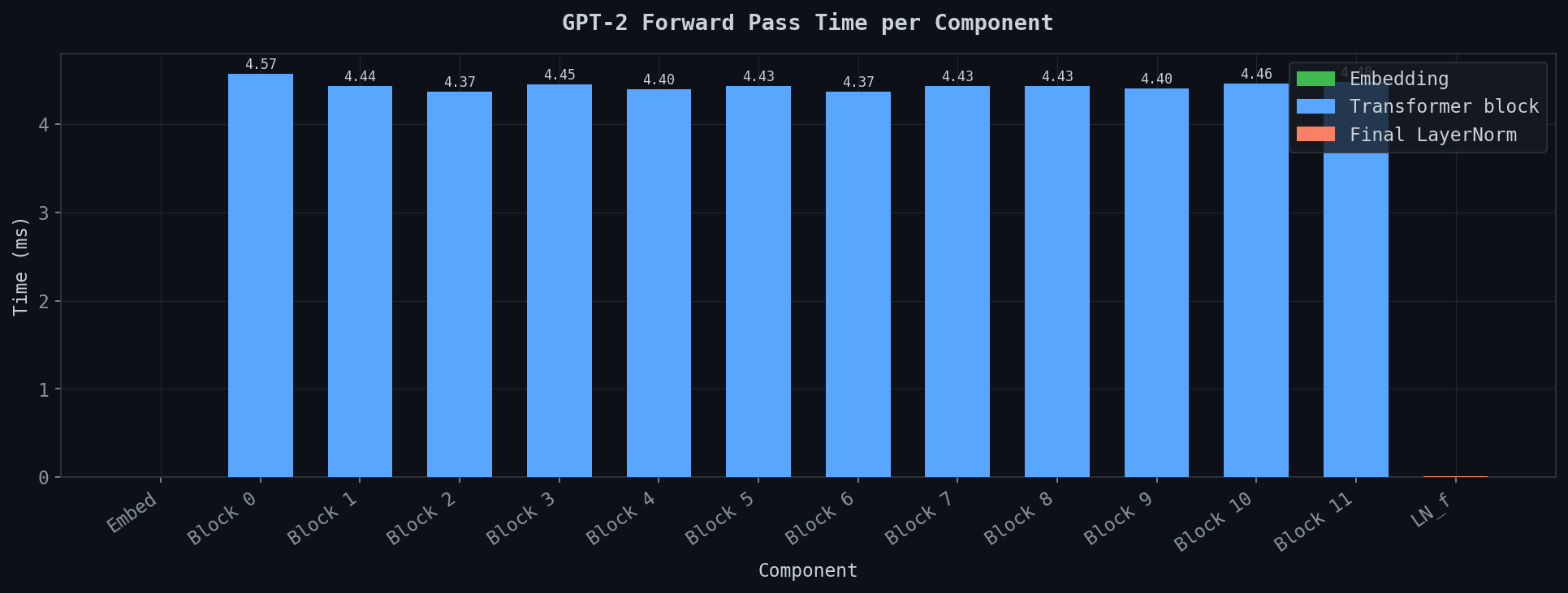
How boring this graph is — and boring is exactly right.
Block 0: 4.57ms. Block 11: 4.46ms. Everything in between: 4.37–4.45ms. Perfectly uniform — same operations, same dimensions, same compute, same time. Layer after layer.
Two things nearly invisible: embedding lookup at the far left, essentially 0ms — it’s a table lookup. Final LayerNorm on the right — a rounding error.
The transformer block is the cost. Everything else is noise.
Attention is O(N²)
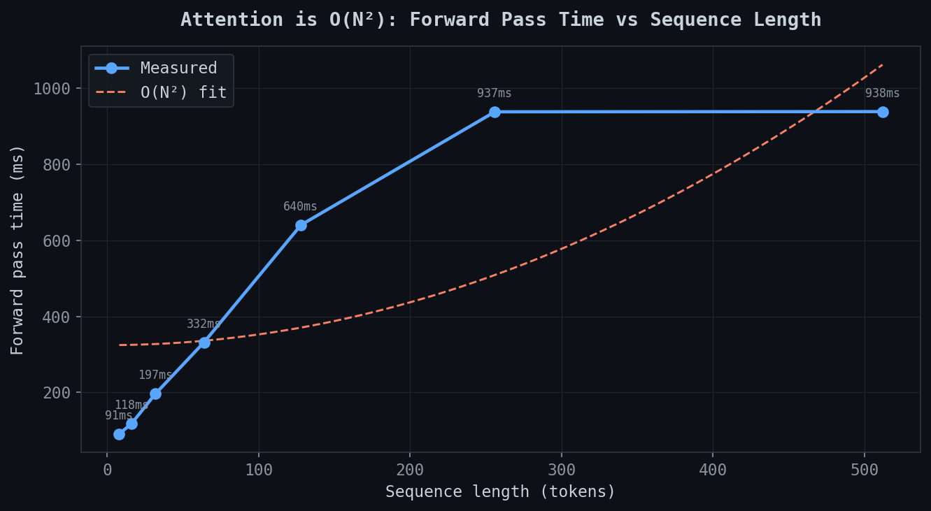
This is the one that matters. This is why long context is expensive.
| Sequence length | Forward pass time |
|---|---|
| 4 tokens | 91ms |
| 8 tokens | 118ms |
| 32 tokens | 197ms |
| 64 tokens | 332ms |
| 128 tokens | 640ms |
| 256 tokens | 937ms |
| 512 tokens | 938ms |
4 tokens to 128 tokens — 32× increase in sequence length — forward pass goes from 91ms to 640ms. Not 32× slower. More like 7×. Already worse than linear.
O(N²) fit overlaid in orange. Measured curve tracks closely up to 256 tokens then flattens — memory bandwidth starts dominating on CPU. But the shape is clear. is [seq, seq]. Double the sequence, quadruple attention compute. Context windows are not free.
This is why FlashAttention exists. Why linear attention exists. Getting manageable at 128K context is not a solved problem.
Top-k sampling distribution
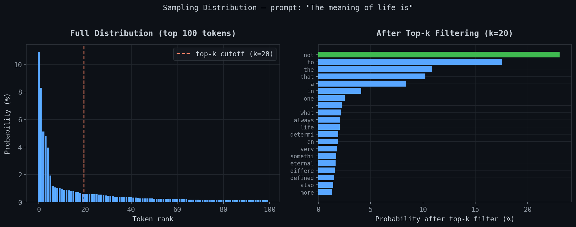
Prompt: “The meaning of life is”
Left: full distribution over top 100 tokens. Steep drop from rank 0 to near-zero by rank 20, then a flat line to rank 100. Top-k cutoff at k=20 is the red dashed line.
Right: after filtering. “not” jumps to ~22%, “to” to ~18%, “the” and “that” around 10%.
The point is the tail. Without top-k, tokens ranked 40-100 have non-zero probability. They’re garbage. Top-k cuts them off and renormalises. The difference between coherent and incoherent output.
Temperature effect
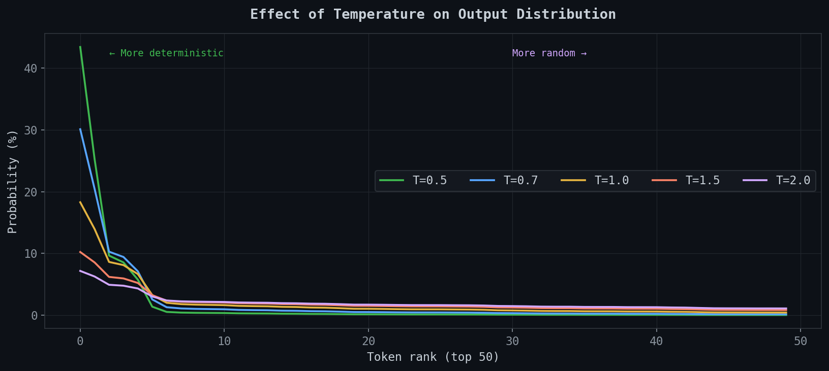
At T=0.5 the top token hits ~44%. At T=2.0 it’s at ~7% — almost flat across the top 50. T=1.0 is what the model was trained at. Below that: more conservative than trained. Above: more chaotic. Neither wrong — depends what you want.
Memory breakdown
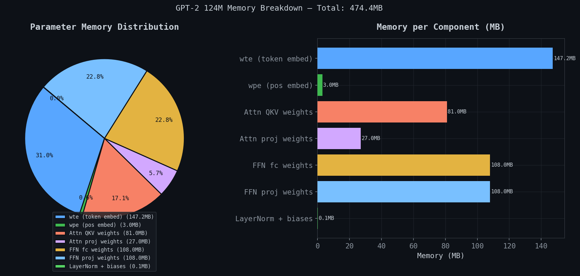
Total: 474.4MB for GPT-2 124M.
| Component | Memory |
|---|---|
| wte (token embeddings) | 147.2MB — 31% |
| FFN fc weights | 108.0MB — 22.8% |
| FFN proj weights | 108.0MB — 22.8% |
| Attn QKV weights | 81.0MB — 17.1% |
| Attn proj weights | 27.0MB — 5.7% |
| wpe (pos embeddings) | 3.0MB |
| LayerNorm + biases | 0.1MB |
Three surprises. First — wte at 147.2MB is 31% of the model. One embedding table. And because of weight tying, this same matrix does double duty as the output classifier — saving another 147MB.
Second — FFN weights (216MB combined) dwarf attention weights (108MB combined). People assume attention is the expensive part. It’s not. The Geva et al. result in practice.
Third — LayerNorm: 0.1MB. The operation that keeps the architecture trainable costs essentially nothing.
Conclusions
Attention is not magic. It’s dot products, softmax, and a weighted sum. The magic is in what the model learns to put in those vectors — query vectors that ask the right questions, key vectors that answer them, value vectors that carry the right information. The mechanism is simple. The learned content is not.
The O(N²) graph is the honest answer to why the field is still actively working on this. A 2017 architecture running on a 2019 pretrained model, on a consumer GPU in 2025, hits a compute wall at a few hundred tokens. Modern systems running 128K context are doing serious engineering to get around that wall — not by fixing the math, but by attacking the memory access patterns.
That’s a GPU problem. Next post: GPU Architecture. Not CUDA yet.
The Code & A Thank You
The full C++ implementation — weight loading, forward pass, tokenization, sampling — is on GitHub: github.com/kailashnagarajan/gpt.cpp. If you’re going to implement this yourself, I’d strongly suggest doing it. Reading about transformers and building one are very different experiences. The Eigen bugs alone will teach you things no blog post can.
I also want to acknowledge something a bit meta. This post was written in genuine collaboration with Claude. Not in the “I asked it to write my blog” way — all the technical substance, the benchmarks, the bugs, the implementations are mine. But Claude was a real partner in drafting and refining the prose, creating the Excalidraw diagrams, building the interactive widgets, and being a sounding board while I was working through the architecture. It’s a strange thing to thank an AI in a blog post about how AI works, but it would feel dishonest not to. The irony of using attention-based models to write about attention-based models is not lost on me.
References
- Vaswani et al. (2017) — Attention is All You Need
- Radford et al. (2019) — Language Models are Unsupervised Multitask Learners (GPT-2)
- Geva et al. (2021) — Transformer Feed-Forward Layers Are Key-Value Memories
- Alammar (2018) — The Illustrated Transformer
- Karpathy — Let’s build GPT from scratch