Multi-Armed Bandits Explained!

Introduction
What is a bandit and multi-arm bandits?
The idea of exploration and exploitation
The multi-armed bandit problem
Algorithms to find the best arm
- Value function based methods
- Upper Confidence Bounds (UCB-1)
Conclusion
References

Introduction

In the past few years reinforcement learning (RL) has impressed computer scientists, mathematicians and laymen alike with its capabilities across various applications. Not only has RL performed close to human behaviour in various tasks — it has exceeded it. One of the best examples is Google DeepMind’s AlphaGo, where the program defeated the world champion of Go 4-1. DeepMind used RL to teach the computer to play Go by learning from thousands of recorded games and letting it play against itself. I believe this was one of the most magnificent feats achieved by humankind in the past decade.

In this blog, I’m not going to talk about anything as fancy as AlphaGo. But I am going to break down some very fundamental ideas in reinforcement learning. This post is inspired by a reinforcement learning course from IIT Madras and heavily by Chapters 1 & 2 of Sutton & Barto.

The aim of this post is to introduce the bandit problem — a simple version of the full RL problem. RL learns about a system by interacting with it and its environment, which is very similar to how humans learn. The idea actually originated in the psychology of animal learning. You can read more about the history of RL here.

What is a bandit and multi-arm bandits?

According to Wikipedia:

“The multi-armed bandit problem is a problem in which a fixed limited set of resources must be allocated between competing choices in a way that maximizes their expected gain, when each choice’s properties are only partially known at the time of allocation.”

Intuitively — you have a system where you pull an arm and get a reward. When you have N such arms, the multi-armed bandit problem asks: what is the best arm (or combination of arms) to pull to maximize reward?

The name “bandit” comes from a gambler pulling the arms of a slot machine. In what sequence should he pull to gain the maximum money? With only one arm, it’s called the “one-arm bandit problem.”

A practical example from the book: You’re faced with $N$ choices and must pick one. After each pick you receive a numerical reward from a random probability distribution depending on your choice. Your goal is to maximize the expected total reward over time.

One interesting real-world application: clinical trials. How can a physician minimize patient loss while investigating the effects of different experimental treatments?

The idea of exploration and exploitation

To maximize reward, two ideas come into tension:

Find which action gives the highest reward.
Use that action as much as possible.

The problem is you must balance these two effectively. If you pick action 2 (reward +5) and exploit it without exploring, you might miss action 15 (reward +10). You’re stuck at a local maximum.

The first idea is called exploration.
The second is called exploitation.

A good balance of both is required to actually maximize expected reward.

The multi-armed bandit problem

Notation

Actions taken at time $t$ : $A_t$
Numerical rewards at time $t$ : $R_t$

The value of picking action $a$ , denoted $q_*(a)$ , is the expected reward given that $a$ is selected:

q_*(a) = \mathbb{E}[R_t \mid A_t = a]

If we knew these values, the problem is trivial — just pick the max. But we don’t, so we work with an estimate $Q_t(a)$ . The goal is to bring $Q_t(a)$ as close as possible to $q_*(a)$ .

What are we optimizing for?

1. Asymptotic Correctness — As $t \to \infty$ , always pick the arm with maximum reward.

2. Regret Optimality — Minimize regret. If you knew the best arm from the start, the difference between that reward and what you actually got is the regret.

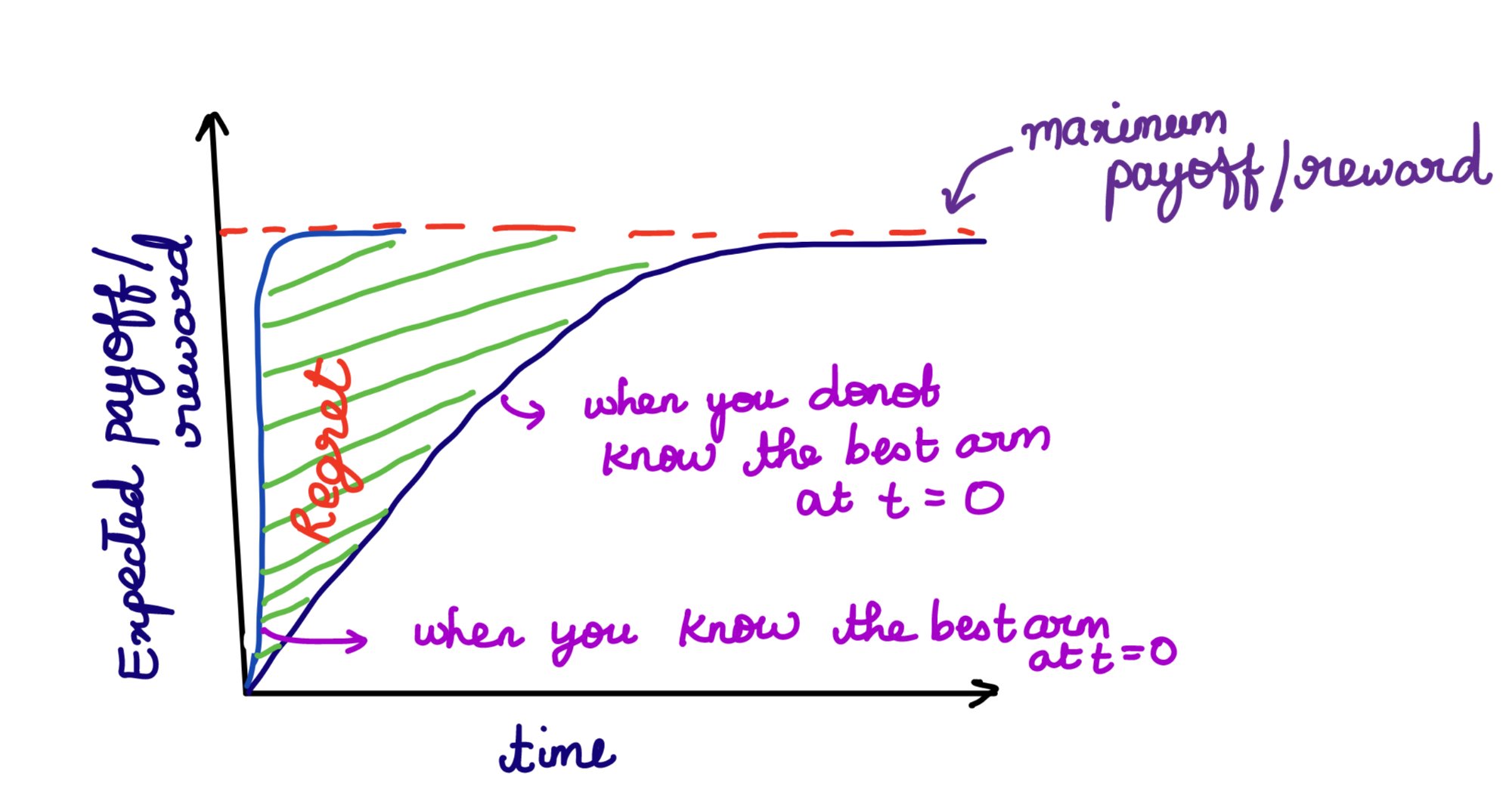Fig 1: Regret Optimality — the shaded region is regret accumulated while learning the best arm.

3. PAC Optimality — Probably Approximately Correct. With probability $1 - \delta$ , the solution should be within $\epsilon$ of the best arm:

P\left(q_*(a) \geq q_*(a^*) - \epsilon\right) \geq (1 - \delta)

The goal: find the minimum number of samples to achieve PAC optimality given $(\epsilon, \delta)$ .

Algorithms to find the best arm

1. Value function based methods

$\epsilon$ -Greedy Algorithm

The estimate of $q_*(a)$ is $Q_t(a)$ , defined as:

Q_t(a) = \frac{\sum_{i=1}^{t-1} R_i \cdot \mathbb{1}_{A_i = a}}{\sum_{i=1}^{t-1} \mathbb{1}_{A_i = a}}

where $\mathbb{1}$ is an indicator function ( $1$ if $A_i = a$ , else $0$ ).

In pure greedy: $A_t = \arg\max_a Q_t(a)$ . This always exploits and never explores — inefficient.

The fix is $\epsilon$ -greedy: be greedy with probability $(1 - \epsilon)$ , explore randomly with probability $\epsilon$ :

A_t = \begin{cases} \arg\max_a Q_t(a) & \text{with probability } (1-\epsilon) \\ \text{uniform sample from } \mathcal{A} & \text{with probability } \epsilon \end{cases}

Problem: The greedy action gets the bulk of probability, all others get equal share regardless of their estimated values.

Softmax Exploration

Fix: make the probability of picking an action proportional to $Q$ :

P(a_t = a) = \frac{\exp\left(\frac{Q_t(a)}{\beta}\right)}{\sum_{b=1}^{n} \exp\left(\frac{Q_t(b)}{\beta}\right)}

$\beta$ is the temperature parameter:

$\beta \to \infty$ : all actions equiprobable
$\beta \to 0$ : greedy selection

To guarantee asymptotic correctness, cool down $\epsilon$ gradually over time.

Food for thought: If rewards come from a stationary distribution and an arm is pulled 1000 times, the 1001st sample has very little effect. Can you adjust rewards to give more weight to recent samples? See pages 32–33 of the book.

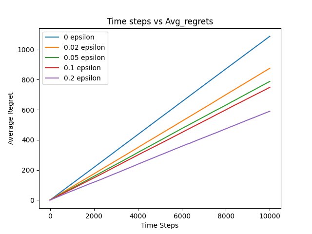Epsilon Greedy Plot Fig 2: Average Regret vs Time steps for different $\epsilon$ values. What can you deduce about asymptotic correctness and regret optimality?

2. Upper Confidence Bounds (UCB-1)

$\epsilon$ -greedy selects non-greedy actions indiscriminately. UCB-1 does better — it selects non-greedy actions based on their potential to be optimal.

Pseudocode:

$k$ arms, $N$ is discrete time
$Q(a)$ is the estimated value of pulling arm $a$
Initialize by pulling each arm at least once
Loop: play arm $j$ that maximizes:

\arg\max_j \left[ Q(j) + \sqrt{\frac{2 \ln n}{n_j}} \right]

The square root term is a measure of uncertainty in the estimate of $Q(a)$ :

As $n_j$ increases (arm $j$ played more), uncertainty decreases
As $n$ increases (more total plays), uncertainty increases for all arms
The $\ln n$ ensures the increase in uncertainty shrinks over time

This ensures all actions are eventually selected, but actions with lower estimates or high play counts are selected with decreasing frequency.

UCB-1 Regret Theorem:

For $k > 0$ , if UCB-1 is run on $k$ arms with arbitrary reward distributions in $[0, 1]$ , the expected regret after $n$ plays is at most:

8 \sum_{i: q_*(i) < q_*(a^*)} \frac{\ln n}{\Delta_i} + \left(1 + \frac{\pi^2}{3}\right) \sum_{j=1}^{k} \Delta_j

where $\Delta_i = q_*(a^*) - q_*(i)$ .

The proof uses Chernoff-Hoeffding (concentration) bounds. See this video for the full derivation.

Limitations of UCB-1:

Hard to extend to non-stationary problems
Difficult to scale to larger state spaces with function approximation

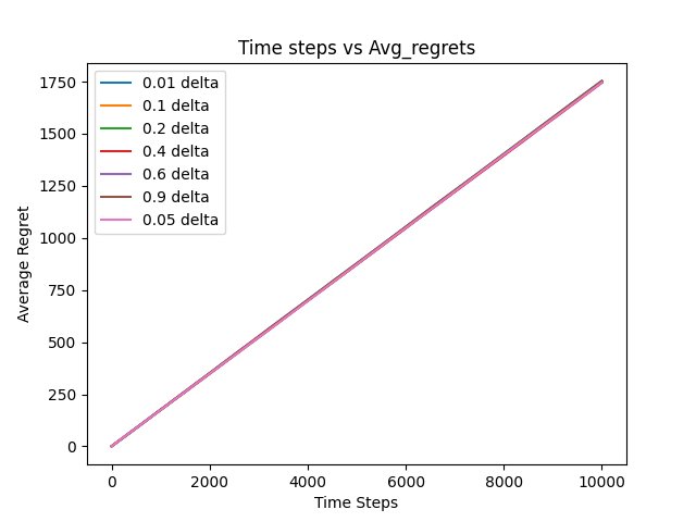UCB Plot Fig 3: Average Regret vs Time steps for UCB-1. What can you deduce about asymptotic correctness and regret optimality?

The code for both algorithms is on my GitHub.

Conclusion

It was a longer post than I expected — I had a lot of fun revisiting my notes and going through the textbook. The MAB problem is a small but important introduction to the full RL problem.

Notice that in the algorithms we discussed, actions have no consequences on future states. There’s no “state propagation model.” That’s far from reality in full RL — where we must consider how an action affects the state and its long-term consequences.

I hope to write at least one more post on RL basics, and eventually implement and write about specific papers.

Table of contents